Introduction
In your last trip to the grocery store, you probably noticed many prices end in “99.” like this one here Food Prices. Why do marketers price products this way instead of rounding prices to the nearest whole dollar? While it may seem surprising, such pricing strategies have been very effective in increasing sales and consequently profits as well, by taking the advantage of the left-digit bias. The left-digit bias describes a phenomenon in which consumer's perceptions and evaluations are disproportionately influenced by the left-most digit of the product price. But when is this bias more likely to exert influence on consumers?
In this article, we will be looking at implementing linear and logistic regression models for detecting the presence of left-digit bias.
Dataset
The dataset used in this post is from course work of Data Driven Marketing. It consists of the attributes of second-hand cars and their sold/unsold status. Due to confidentiality issues, the original features were transformed and shifted. The features given in the dataset consists of 7 independent variables. 'Mile' is the number of miles the car had travelled and the 'Price' refers to the selling price of the car. The response variable, ‘Sold’ is a binary variable indicating 1 for a sold car and 0 otherwise.
Approach
The objective is to detect the presence of left-digit bias or not when the customer plans to purchase a car. In Machine Learning terms, this is a classification problem. Here, we will implement a logistic regression model
Logistic Regression
Logistic regression is a type of classification algorithm which is being used since early twentieth century. The algorithm tries to find relationship between the features and probability of a particular outcome. Logistic regression is further divided into various sub-types – binary, multinomial, ordinal; depending upon the type of response variable. In this post, we will build a binary logistic model as our response variable is binary - ‘Sold’ or ‘Not Sold’.
Data Preparation
We will prepare our data for training. Load the required libraries and read the csv file. You can download the dataset from here.
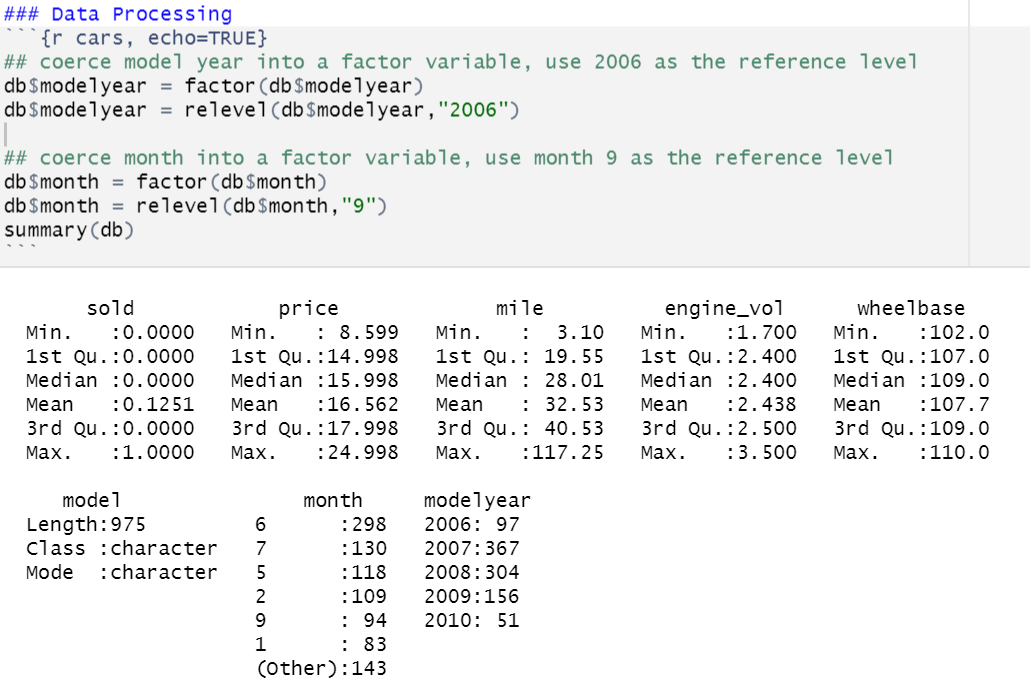
As discussed before there are 7 independent variables, but we have modelyear and month as factor variables. We set a base for these factor variables and proceed to make the model. Class is our response variable. There are 975 rows and 8 columns.
Let’s look at missing values and the proportion of classes.
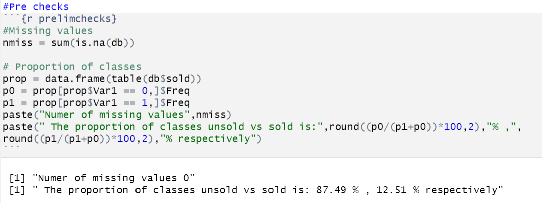
Woah! 853 out of 975 observations (87.5%) of the data is of class ‘Not Sold’.
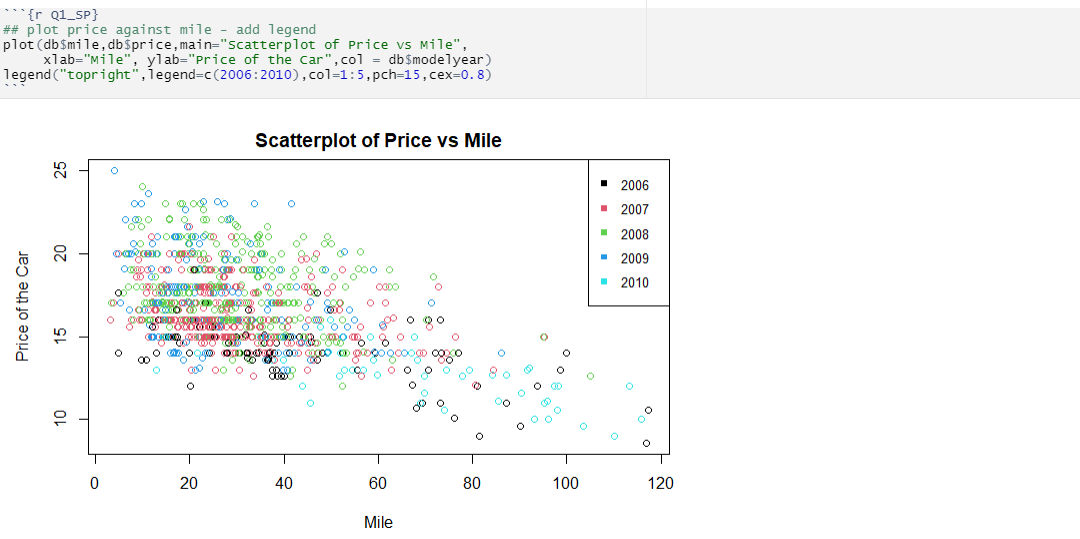
Price vs Mile Relationship
Now let us analyze the relationship between Price vs Mile. We have observed that, the above plot shows that the price of the car declines with the increase in the number of miles traveled. It also shows that the there are a lot of cars with similar selling price i.e. horizontal lines even though the mileage is different and that's because mileage is not the only factor affecting the price.
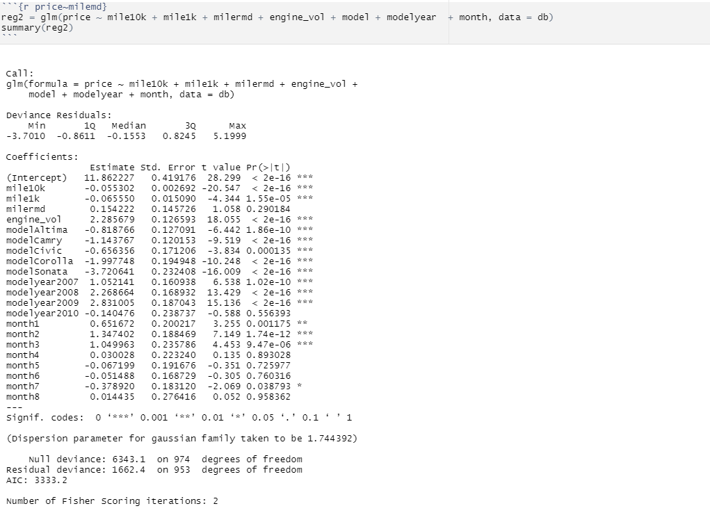
Let us decompose the mile into thousands, tens and decimals.
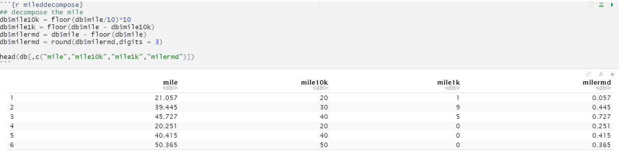
Let us check if every component of mile is significant when we set the price based on these values. So we fit a linear regrssion model to predict price with all the decomposed mile variables We can infer that the left digits of the decomposed price (mile10k, mile1k) behave in a similar way that of the mile in the first scatter plot (Negative Coefficient for Estimate). But last mile digits (milermd) are positively affecting the price and not significant enough to predict the price ("Pr(>|z|)" = 0.290184) while the left ones are significant with almost 100% ("Pr(>|z|)" < 0.001)
Sold vs Price Relationship
Let’s decompose the price similar to mile and build a logistic regrssion model with 7 features and test the significance of the decomposed prices
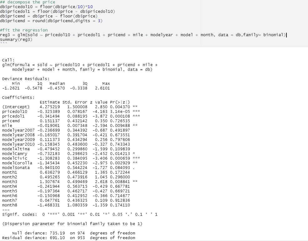
What do the coeffecients of the decomposed price variables indicate?
After observing the results of the above model, we can say that the left digit bias is evident for sold vs decomposed price, because the left digits (pricedol10, pricedol1) are significant with almost 100% confidence ("Pr(>|z|)" < 0.001) whereas the right most ones (pricemd) aren't significant enough to predict the selling probability ("Pr(>|z|)" = 0.726535).
Inferences
We can conclude that the left digit bias exists when a consumer is trying to purchase a used car. Therefore, the store managers can be more proactive while setting a price for the car i.e. they can increase the last digits part of the price for more profit margin.
But left digit bias can be across multiple variables i.e. in the above example, it is price and miles. But both these variables can be interdependent with each other. So the store managers can take the left digit bias into account, but focus on the most important variable to apply this left digit bias.
Thanks for reading this :). Let me know you thoughts about this article in the comments!